
A phase transition of first order occurs, when the free-energy of a thermodynamical system F(T,V,N), with temperature T, volume V and particle number N, has two local minima. This means, that the system has two different homogeneous equilibrium states. These minimima are then necessarily divided by an energy barrier, that is, a region of concave F. This has the immediate consequence, that there is a certain region V I < V < V II in which a homogeneous state is energetically disadvantageous compared to a heterogeneous state, where the system’s material is divided into coexisting parts with the densities nI = N∕V I and nII = N∕V II. Realizations of such heterogeneous states are commonly observed, for example, in the liquid/vapour transition of H2O or CO2, where the coexistence of liquid and vapour can readily be prepared experimentally.
In order to illuminate this phenomenon, we will first determine the boundaries of the coexistence region V I,V II and then calculate the free-energy of the heterogeneous state.
In equilibrium, the coexistence of two phases is possible if and only if pressure p, temperature T, and chemical potential μ are equal in both phases, that is, throughout the entire system. Therefore, one can use the condition
|
|
where pI∕II denotes the coexistence pressure, together with the Gibbs-Duhem relation G = ∑ jμj, with free enthalpy G, to infer
| GI(T,pI∕II) = GII(T,pI∕II) | |||
| ⇔ FI + pI∕IIV I = FII + pI∕IIV II | |||
⇒ FI − FII = pI∕II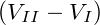 . . | (1) |
 | (2) |
we can combine the equations (1) and (2) to obtain
 |
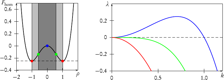
This result allows to find the coexistence region by a simple geometrical approach: the famous Maxwell construction. Drawing the isotherm of the homogeneous system in a pressure-volume diagram, the coexistence pressure pI∕II corresponds to a horizontal line which is drawn in a way that the areas A and B in Fig. 1 are of equal size. This uniquely defines pI∕II, V I, and V II.
The energy of the heterogeneous state is given by F = cIFI + cIIFII, where FI = F(T,V I,N) and FII = F(T,V II,N) while cI = NI∕N and cII = NII∕N denote the fractions of molecules in the two phases. Since cI + cII = 1 and V = cIV I + cIIV II, we can deduce the so-called lever rule:
 |
Accordingly, we can write the free-energy of the heterogeneous state as
 |
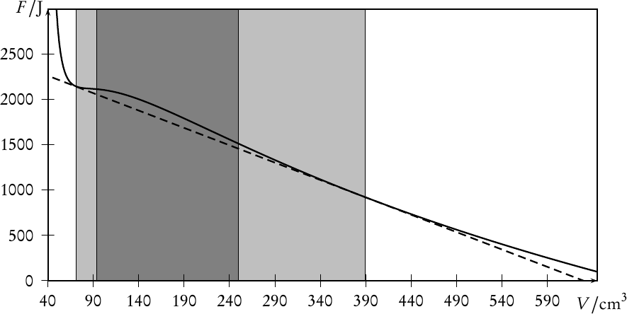
which is obviously a straight line with the slope ∂Fhet∕∂V = (FII −FI)∕(V II −V I), connecting F(T,V I,N) and F(T,V II,N). Since we argued above, that the pressure p = −∂F∕∂V is constant along any isotherm in the coexistence region, we infer that the straight line Fhet is actually tangent to F in both points F(T,V I,N) and F(T,V II,N). It is thus termed the common tangent in the literature. Due to the concavity of the free-energy of the homogeneous state in between the two local minima, the tangent Fhet is lying below F, making the heterogeneous states on the tangent energetically more favourable. This is shown graphically in Fig. 2.
This region in state-space in which the heterogeneous state has a lower overall free-energy is called the binodal region, and it is the region where phase coexistence is possible. Its boundary, the binodal curve, is given by the loci of V I,V II written as functions of another state variable such as the temperature T, yielding curves V I(T),V II(T). If phase coexistence is not possible for all values of T, then the two curves V I(T),V II(T) will meet in a critical point at a temperature Tcr beyond which the phases are no longer distinguishable from each other.
However, the given argument does not claim that a state within the binodal is unstable but only that it is metastable, that is, unstable to finite but not to infinitesimal perturbations. In fact, these metastable states are commonly observed, for example in form of an overheated liquid or an undercooled gas.
So, when does the homogeneous state actually become unstable? Looking at the pressure p = −∂F(T,V,N)∕∂V of the system, we note that any state with ∂p∕∂V = −∂2F∕∂V 2 > 0, is mechanically unstable, so that the inflection points ∂2F(T,V,N)∕∂V 2 = 0, when written as functions of another state variable, such as T, demark a boundary, the so-called spinodal curve beyond which no homogeneous state can exist. The region within this boundary, that is the region of negatively curved F(T,V,N), is called the spinodal region. In the next subsection, we will explain this instability by use of an energetic argument.
It is clear that the spinodal region is a subset of the binodal region, since in between every two minima of the free-energy there is necessarily a region of negative curvature. By the same argument, we can deduce that spinodal and binodal meet in the critical point, because the minima smoothly approach each other for T → Tcr, so that minima and inflection points finally coincide.
Throughout this thesis, we will describe the surfactant monolayer in terms of its
molecular number density n = N∕V . We therefore use the remainder of
this subsection to formulate the free-energy using the variable n, that is
 (T,V,n) := F(T,V,nV ), and write
 | (3) |
denoting the system’s free-energy density by f(T,n).
The pressure of the system is then given by
p = − | = − − −  | ||
= − + +   | |||
= − + nμ, + nμ, |
 | (4) |
In order to determine the mechanical stability of homogeneous states, we have to calculate
 = = |  − −  | ||
= − − 2 − 2  | |||
−  . . |
 |
yielding
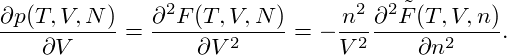 |
We conclude that, no matter if we look at the free-energy in terms of variable volume V or variable density n, the stability is always determined by the second derivative of the corresponding free-energy function.
The conditon of mechanical stability, ∂p(T,V,N)∕∂V < 0, can be substantiated by a simple energetical argument which, despite its illustrativeness, is - at least to the author’s awareness - never given in the literature.
A homogeneous state is unstable when even an infinitesimal perturbation leads to a state of lower free-energy. Let us assume, that an initially homogeneous system of density n0 is perturbed with a perturbation of amplitude dn, so that a volume portion V + of the fixed total volume V 0 now has the density n0 + dn with infinitesimal dn. Material conservation demands, that another portion V 0 − V + is perturbed at the same time so that it now has the density n0 − V +∕(V 0 − V +)dn. Then the free-energy difference between the perturbed and the initial state is given by
| ΔF | = V +f(n0 + dn) + (V 0 − V +)f − V 0f(n0) − V 0f(n0) | ||
= (V + − V 0)f(n0) + V +  n
0dn + V + n
0dn + V +  dn2 dn2 | |||
+ (V 0 − V +)![[ ]
∂f V+ 1 ∂2f ( V+ )2 2
f (n0)− ∂n|n0V-−-V--dn− 2 ∂n2|n0 V--−-V- dn
0 + 0 +](spinodal33x.png) | |||
+   . . |
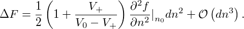 |
Since V + is by definition positive and less than V 0, we conclude that the sign of ΔF for infinitesimal dn is determined solely by the curvature of the free-energy density in the inital state n0. Note, that the above argument holds true also when we assume the perturbation to be limited to a subvolume V ′⊂ V 0. This means, that a local infinitesimal fluctuation around n0 will reduce the free-energy of the system if and only if ∂2f(n0)∕∂n2 < 0. Thus, we have reproduced the stability conditon given in the previus section by explicitly referring to the change of the system’s free-energy.
So far we have only considered equilibrium states and investigated their stability. The actual dynamics of a system within the spinodal region is governed by the Cahn-Hilliard equation [CH58], which describes the time evolution of the spatially varying density ρ(x,t) of the considered thermodynamical system. It can be written as a conservation law
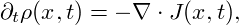 |
with the flux
![-δF-[ρ]-
J(x,t) = − α ∇δρ(x,t),](spinodal37x.png) | (5) |
where α denotes a mobility factor. In the simple case of constant α, the Cahn-Hilliard equation takes the form
![-δF-[ρ]-
∂tρ(x,t) = α Δδρ(x,t).](spinodal38x.png) | (6) |
It is important to recognize, that the Cahn-Hilliard equation exhibits potential
dynamics. This means that an isolated system approaches an equilibrium state, which
corresponds to a local minimum of the free-energy functional  [ρ]. In the
terminology of nonlinear dynamics this means, that [ρ] is the Lyapunov functional
of the system.
[ρ]. In the
terminology of nonlinear dynamics this means, that [ρ] is the Lyapunov functional
of the system.
This holds true for arbitrary positive definite mobility factors. To prove
this, one has to consider how [ρ] changes with time. A short calculation
yields
| ∂t | = ∫
V dDx ∂tρ(x) ∂tρ(x) |  insert (6) insert (6) | |||||
= ∫
V dDx ∇⋅ ∇⋅![[ ]
α∇ -δF--
δρ(x)](spinodal42x.png) |  int. by parts int. by parts | ||||||
= ∫
V dDx∇![[ δF δF ]
αδρ(x)∇ δρ(x)-](spinodal44x.png) −∫
V dDxα −∫
V dDxα 2 2 |  Gauss’ law Gauss’ law | ||||||
= ∫
∂V d(D−1)xα ∇ ∇ −∫
V dDxα −∫
V dDxα 2. 2. |
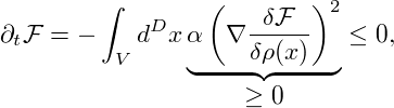 | (7) |
that is, either ρ is already in an equilibrium state or it is evolving towards one.
Cahn and Hilliard proposed the following free-energy functional for a general isotropic system of nonuniform composition [CH58]:
![∫ { κ }
F[ρ] = dDx --(∇ ρ)2 + fhom (ρ) .
V 2](spinodal51x.png) | (8) |
The idea behind this model is simple: To molecules within a subvolume dV of the
system it makes little difference whether they are part of a homogeneous system or of
an inhomogeneous system with very small density gradients. Thus, as a zeroth
approximation, the system’s overall free-energy simply equals the sum of
the free-energies of each infinitesimal subvolume, fhom(ρ( ))dV . One can
expand the free-energy density in powers of ∇ρ, keeping only the lowest
orders:
))dV . One can
expand the free-energy density in powers of ∇ρ, keeping only the lowest
orders:
 |
The tensors κ(1,2) and the vector L reflect the symmetry properties of the considered material. For isotropic media, one obtains L = 0 and κ(1) = κ1I, κ(2) = κ2I, yielding the free-energy density of eq. (8), where κ = −dκ1∕dρ + κ2∕2.
Inserting the free-energy functional (8) into the Cahn- Hilliard equation (6), we obtain
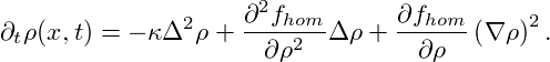 | (9) |
From our considerations in section 1 we already know qualitatively what to expect from solutions to this equation: Homogeneous system outside of the binodal region are absolutely stable, within the binodal region they are metastable, and in the spinodal region they are unstable. Upon instability, the homogeneous state decomposes into coexisting domains of different densities ρI, ρII.
Spatially homogeneous fields ρ =  = const. are always stationary solutions of the
Cahn-Hilliard equation. The linear stability of these solutions is readily obtained by
looking at small perturbations ζ(x,t). Inserting ρ(x,t) =
= const. are always stationary solutions of the
Cahn-Hilliard equation. The linear stability of these solutions is readily obtained by
looking at small perturbations ζ(x,t). Inserting ρ(x,t) =  + ζ(x,t) into eq. (9), and
keeping only the linear terms, we find that the time evolution of the perturbation is
governed by
+ ζ(x,t) into eq. (9), and
keeping only the linear terms, we find that the time evolution of the perturbation is
governed by
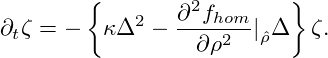 |
Using the ansatz ζ ∼ exp(λt + ik ⋅ x), one finds the dispersion relation of the perturbation, which only depends on the absolute value of the wavevector k = |k|, since only even powers of ∇ are applied to ζ:
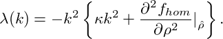 | (10) |
From this expression, it is obvious, that the stability of a homogeneous solution
 is determined by the curvature of the free-energy at ρ =
  . Physically
speaking, a solution
. Physically
speaking, a solution  is stable, as long as it is chosen from outside the spinodal
region, which is defined as the region of concave fhom. Dispersion relations for
three different
is stable, as long as it is chosen from outside the spinodal
region, which is defined as the region of concave fhom. Dispersion relations for
three different  in a system with a free-energy of symmetric double-well
shape are shown in Figure 3. Otherwise, there is finite band of modes k
with 0 < k <
in a system with a free-energy of symmetric double-well
shape are shown in Figure 3. Otherwise, there is finite band of modes k
with 0 < k <  which are amplified with λ(k) > 0. The
wavenumber kmax, which is maximally amplified, can be calculated from eq. (10)
as
which are amplified with λ(k) > 0. The
wavenumber kmax, which is maximally amplified, can be calculated from eq. (10)
as
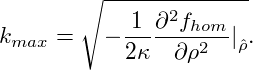 |
The corresponding maximal amplification is given by
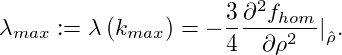 |
With kmax and λmax we have obtained an estimate of the inverse time and length scales of the early stages of spinodal decomposition.
However, after a short time, the nonlinearity of eq. 9 strikes and leads to a different behaviour known as coarsening of the domains which are formed during the initial pattern formation. During this process, large domains grow larger while small domains grow smaller and finally disappear. Two mechanisms can be distinguished: Firstly, two domains can directly merge into a single larger one, thereby minimizing thier overall interfacial energy. Secondly, material diffuses from the surface of small domains towards the larger ones, that is, the domains are absorbed without direct contact to other domains. This phenomenon is known as Ostwald-ripening.
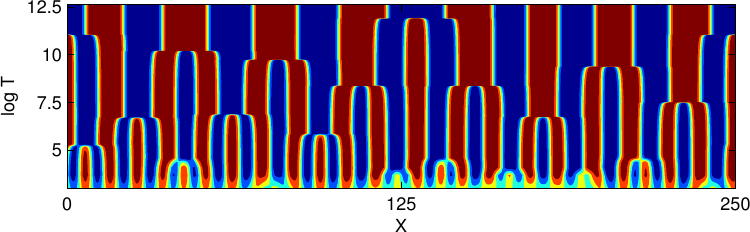
Figure 4 visualizes the dynamics of this process in a spacetime plot. The domain shape depends on the amount of available material. The phase with the smaller overall volume will form spherical domains in order to diminish the interfacial energy. If, however, both phases have roughly the same total volume, one will rather observe labyrinthine structures. The coarsening process will continue, until finally only one domain of each phase remains, divided by the smallest possible interface.
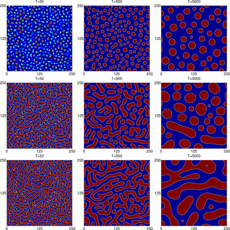
 = −0.4, in the second row
  = −0.1, and in the third row
  = 0.
In each row, time increases from left to right. The coarsening of the structures
towards higher average wavelength can be clearly seen. Comparing the pictures
of each column, one can see the different morphologies of the resulting patterns,
going from circular domains to labyrinthine patterns as
= 0.
In each row, time increases from left to right. The coarsening of the structures
towards higher average wavelength can be clearly seen. Comparing the pictures
of each column, one can see the different morphologies of the resulting patterns,
going from circular domains to labyrinthine patterns as  → 0.
→ 0.